Getting started

First step: loading the data cube

# import base class for the manipulation of a SITELLE spectral cube: SpectralCube
from orcs.process import SpectralCube
import pylab as pl

cube = SpectralCube('/home/thomas/M31_SN3.merged.cm1.1.0.hdf5')

master.ff2bd|INFO| Cube is level 3
master.ff2bd|INFO| shape: (2048, 2064, 840)
master.ff2bd|INFO| wavenumber calibration: True
master.ff2bd|INFO| flux calibration: True
master.ff2bd|INFO| wcs calibration: True

## Resetting flux calibration
# You should not do this if your cube has been freshly reduced. The cube used here as an example has an outdated flambda parameter
# which can be reset to the latest one this way.
# Note that this calibration is computed from known instrumental parameters for ideal atmosheric conditions and modulation efficiency.
# The measured flux may thus be underestimated by more than 10%. But, in case something's really wrong in the calibration, this is a good starting point
# which sould not be more than 15% off (and is generally around 5% off).
cube.set_flambda(cube.compute_flambda())

master.ff2bd|INFO| mean flambda config: 1.4984303888958248e-16
master.ff2bd|INFO| standard_spectrum not set: no relative vector correction computed
master.ff2bd|INFO| standard_path not set: no relative vector correction computed
master.ff2bd|WARNING| bad WCS in header
master.ff2bd|INFO| standard_image not set: no absolute vector correction computed

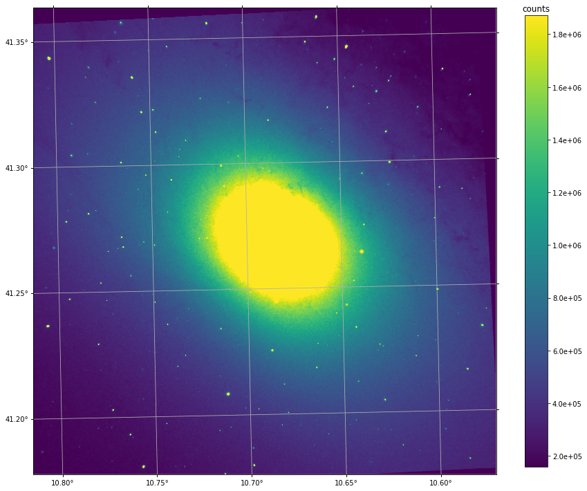
Exploring the deep frame

The deep frame is the sum of all the interferogram frames, i.e. an image of the field with an exposure time of

cube.params.exposure_time * cube.dimz # s

Deep frames for old cubes

Note: if your cube is old (level 1), the deep frame may have been distributed as a separate FITS file. For more recent cubes, the deep frame must be stored in the hdf5 archive. The deep frame is in the cube if one of the following return True:

cube.has_dataset('deep_frame') # should return True
hasattr(cube, 'deep_frame')

If your deep frame was distributed as a separate file, you can attach it to the cube with

cube.deep_frame = orb.utils.io.read_fits('path_to_your_deep_frame.fits')

# explore the deep frame (in counts)
deep = cube.get_deep_frame() # this step should take a second or less. If it takes a lot of time, see above.
deep.imshow(perc=95, wcs=True)
pl.grid()
cb = pl.colorbar(shrink=0.8, format='%.1e')
cb.ax.set_title('counts')
deep.to_fits('M31_SN3.deep_frame.fits') # if you want to exampine it your way (e.g. with ds9 :P)

master.03e73|INFO| Data written as M31_SN3.deep_frame.fits in 0.17 s

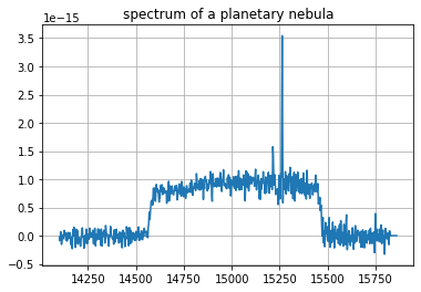
Spectrum extraction and visualization

# extract and plot a spectrum at x=919 y=893 integrated over a radius of 2 pixels
spectrum = cube.get_spectrum(919, 893, 2) # option mean_flux
spectrum.plot(plot_real=True)
pl.grid()
pl.title('spectrum of a planetary nebula')

pl.figure()
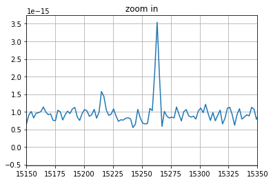
spectrum.plot(plot_real=True)
pl.xlim((15150, 15350))
pl.title('zoom in')
pl.grid()

The returned spectrum is a RealSpectrum object which provides many internal methods, one of which is the ability to fit directly.

• plot: spectrum.plot (by default the real and the imaginary part of the spectrum are displayed, but you can dispaly only the real part with the option: plot_imag=False)

• fit: spectrum.fit

If you want to get the data and the corresponding axis as numpy.ndarray you can do it this way :

• data: spectrum.data

• axis: spectrum.axis.data

print('object type:', spectrum)
print('data as numpy.ndarray vector', type(spectrum.data))
print('axis (in cm-1) as numpy.ndarray vector', type(spectrum.axis.data))

object type: <orb.fft.RealSpectrum object at 0x7f23c82dc350>
data as numpy.ndarray vector <class 'numpy.ndarray'>
axis (in cm-1) as numpy.ndarray vector <class 'numpy.ndarray'>

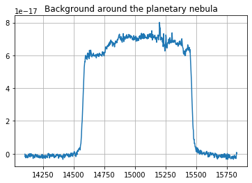
Background removal

background = cube.get_spectrum_in_annulus(919, 893, 4, 25, median=True, mean_flux=True)
# mean_flux=True: The mean flux is returned (i.e. integrated flux / number of integrated pixels).
#  This is important when computing a sky spectrum.
#
# median=True: When combining spectra, the median is used instead of the mean (if mean_flux is True,
#  the computed median vector is then multiplied by the number of integrated pixels to keep with a
#  measure of the total flux.). On large integrated regions, this operation removes outliers like
#  isolated bright stars.
background.plot()
pl.grid()
pl.title('Background around the planetary nebula')

master.03e73|WARNING| /home/thomas/miniconda2/envs/orb3/lib/python3.7/site-packages/numpy/lib/nanfunctions.py:994: RuntimeWarning: All-NaN slice encountered
  result = np.apply_along_axis(_nanmedian1d, axis, a, overwrite_input)

Text(0.5, 1.0, 'Background around the planetary nebula')

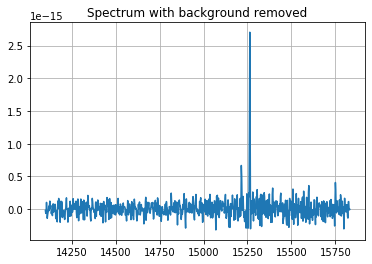
# Background is high below the source. It can be removed by subtracting the spectrum of a region in a an annulus around the source.

spectrum_corr = spectrum.subtract_sky(background)
# note that you didn't have to bother with the number of integrated pixels in each spectrum
# (even if both have been integrated over different surfaces)
spectrum_corr.plot()
pl.grid()
pl.title('Spectrum with background removed')

Text(0.5, 1.0, 'Spectrum with background removed')

Second step: fitting the spectrum

• The emission lines to fit are passed by name (their wavenumber, in cm-1, could also be given directly). Remember that:

\(\sigma [\text{cm}^{-1}] = \frac{1e7}{\lambda [\text{nm}]}\)

• The line model is sinc by default because the instrumental line shape is a sinc. Note that the observed emission line shape is the convolution of its real shape (e.g. a gaussian at a moderate resolution) and the instrumental line shape. i.e., fitting a sinc means that the observed emission line shape is considered a dirac (infinitely narrow line) with respect to the resolution.

python   fmodel = 'sinc'

• The velocity of the lines is -513 km/s. It is passed with the argument:

python   pos_cov = -513,   pos_def = ['1','1']

The velocity is considered as a covarying parameter. By default all the lines are considered to have a free velocity parameter. If we want to set the same velocity to all the lines we must set the definition of the position of eachline to the same covaying group with pos_def = ['1','1'].

• By default the calculated spectrum is multiplied by the filter function. But this can sometimes lead to strange results if no backgound is present. In this case the following option must be set:

python   nofilter = True

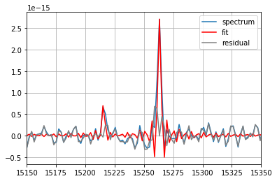
fit = spectrum_corr.fit(['Halpha', '[NII]6583'],
                        fmodel='sinc',
                        pos_cov=(-513,),
                        pos_def=['1', '1'],
                        nofilter=True)
# fitting results are combined into an orb.fit.OutputParams object which behaves exacly like a dict but offers some valuable methods
# for quick results plotting

print(fit) # print the most important results

spectrum_corr.plot(label='spectrum')

fit.plot(label='fit', c='red') # plot the fitted vector
fit.plot_residual(label='residual', c='gray') # plot the residual of the fit
pl.grid()
pl.xlim((15150, 15350))
pl.legend()




# note that more can be retrived by looking into all the data provided:
# print(dict(fit))

=== Fit results ===
lines: ['H3', '[NII]6584'], fmodel: sinc
iterations: 41, fit time: 6.40e-02 s
Velocity (km/s): [-508.1(1.1) -508.1(1.1)]
Flux: [3.03(12)e-15 7.6(1.3)e-16]
Broadening (km/s): [nan +- nan nan +- nan]

<matplotlib.legend.Legend at 0x7f23c0792610>

Ungroup the velocity parameter

We can ungroup the velocity of the emission lines by giving each line a unique group label. We can set:

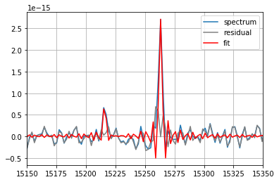
pos_def=['1', '2']

I this case the measured velocity must be different for both lines. But the precision will also be worsen.

fit = spectrum_corr.fit(['Halpha', '[NII]6583'],
                   fmodel='sinc',
                   pos_cov=(-513, -513),
                   pos_def=['1', '2'],
                   nofilter=True)
print(fit)
spectrum_corr.plot(label='spectrum')
fit.plot_residual(label='residual', c='gray') # plot the residual of the fit
fit.plot(label='fit', c='red') # plot the fitted vector

pl.grid()
pl.xlim((15150, 15350))
pl.legend()

=== Fit results ===
lines: ['H3', '[NII]6584'], fmodel: sinc
iterations: 49, fit time: 6.91e-02 s
Velocity (km/s): [-507.6(1.2) -516.3(4.5)]
Flux: [3.04(12)e-15 7.8(1.2)e-16]
Broadening (km/s): [nan +- nan nan +- nan]

<matplotlib.legend.Legend at 0x7f23c06aaa50>

using a sincgauss model with a single broadening parameter

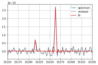
We can try the broadened sincgauss model (sinc instrumental function convoluted with a gaussian). We can group the broadening parameter of the emission lines by giving the same group label to the lines. We can set:

python   fmodel='sincgauss',   sigma_def=['1', '1'],   sigma_cov=20

I this case the measured broadening will be the same for both lines and the precision of the estimations are better. Note that the broadening must be initialized to a nonzero value for the fit to work sigma_cov=20

fit = spectrum_corr.fit(
    ['Halpha', '[NII]6583'],
    fmodel='sincgauss',
    pos_cov=(-513,),
    pos_def=['1', '1'],
    sigma_def=['1', '1'],
    sigma_cov=(20,),
    nofilter=True)
print(fit)
spectrum_corr.plot(label='spectrum')
fit.plot_residual(label='residual', c='gray') # plot the residual of the fit
fit.plot(label='fit', c='red') # plot the fitted vector

pl.grid()
pl.xlim((15150, 15350))
pl.legend()

master.03e73|WARNING| please set a guess, or a covarying value of sigma > 0 or use a  sinc model or you might end up with nans

=== Fit results ===
lines: ['H3', '[NII]6584'], fmodel: sincgauss
iterations: 37, fit time: 1.20e-01 s
Velocity (km/s): [-506.9(1.4) -506.9(1.4)]
Flux: [4.43(24)e-15 1.14(16)e-15]
Broadening (km/s): [27.1(1.7) 27.1(1.7)]

<matplotlib.legend.Legend at 0x7f23c06b3b50>

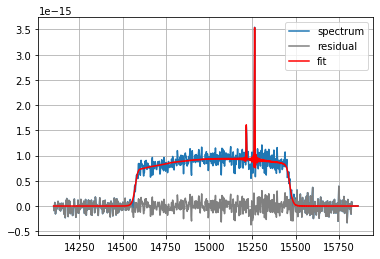
Model with a high background

When the background is high (e.g. it cannot be subtracted or we are fitting emission lines of a high redshift galaxy), we can fit the backgound as a polynomial multiplied by the filter function. The order of the polynomial can be set with poly_order keyword.

fit = spectrum.fit(
    ['Halpha', '[NII]6583'],
    fmodel='sincgauss',
    pos_cov=(-513,),
    pos_def=['1', '1'],
    sigma_def=['1', '1'],
    sigma_cov=(20,),
    nofilter=False,
    poly_order=2)
print(fit)
spectrum.plot(label='spectrum')
fit.plot_residual(label='residual', c='gray') # plot the residual of the fit
fit.plot(label='fit', c='red') # plot the fitted vector

pl.grid()
pl.legend()

master.03e73|WARNING| please set a guess, or a covarying value of sigma > 0 or use a  sinc model or you might end up with nans

=== Fit results ===
lines: ['H3', '[NII]6584'], fmodel: sincgauss
iterations: 55, fit time: 1.96e-01 s
Velocity (km/s): [-507.3(1.4) -507.3(1.4)]
Flux: [4.34(23)e-15 1.13(16)e-15]
Broadening (km/s): [26.6(1.7) 26.6(1.7)]

<matplotlib.legend.Legend at 0x7f23c06c7250>