Introduction ¶

Contents

Introduction

A few words on ORCS ¶

ORCS is a Python module which gives you the keys to the analysis of your SITELLE data cube.

It is composed of calibration methods, extracting tools and a powerful fitting engine specifically designed for interferometric data. When fitting spectra, both a classical (frequentist) and a Bayesian paradigm are available.

Outputs ¶

ORCS generates a lot of different output maps when fitting entire regions of the cube.

File name format is:

[ObjectName]_[Filter].LineMaps.maps.[Lambda]_[ComponentNumber].[Binning].[Parameter].fits

Parameters are:

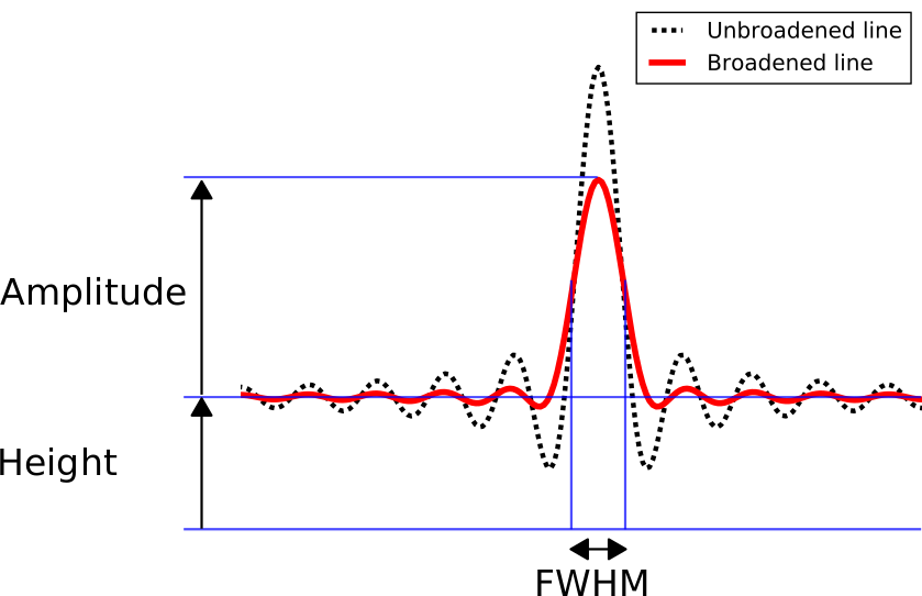
amplitude: Amplitude in erg/cm2/s/A
flux: Integrated flux in erg/cm2/s
height: Height of the continuum below in erg/cm2/s/A
fwhm: FWHM in cm-1 (must be first converted in Angstrom to compute flux in erg/cm2/s)
velocity: Doppler velocity in km/s
sigma: line broadening (with sincgauss model) in km/s (must first be converted in Angstrom to compute flux in erg/cm2/s)

How flux is computed?¶

For a line of amplitude a, width \(\Delta\sigma\) , wavenumber \(\sigma\)

sinc model:

orb.utils.spectrum.sinc1d_flux()¶

\[F = \frac{a \times \text{FWHM}}{1.20671}\]

sincgauss model (D is the Dawson integral):

orb.utils.spectrum.sincgauss1d_flux()¶

\[ \begin{align}\begin{aligned}B = \frac{\sigma}{\sqrt{2}\Delta\sigma}\\F = \frac{\pi a \sigma}{\sqrt{2}}\frac{e^{B^2}}{iD(iB)}\end{aligned}\end{align} \]

Useful conversions ¶

To convert the fwhm or width ( \(\Delta\lambda\) ) to nm from cm-1:

orb.utils.spectrum.fwhm_cm12nm()¶

\[\Delta\lambda [\text{nm}] = \frac{10^7 \Delta\sigma [\text{cm}^{-1}]}{\sigma^2}\]

To convert from FWHM to width for a sincgauss:

\[\Delta\sigma = \frac{\text{FWHM}}{1.20671\pi}\]

To convert broadening from km/s to a shift in cm-1:

orb.utils.fit.vel2sigma()¶

HDF5 Cubes formatting (levels)¶

As ORCS results of years of development, there are different levels of HDF5 cube depending on the moment when the data was obtained and reduced. Each one with a different internal formatting. Note that this concerns you only if you want to access the raw internal data since it should be transparent if you use orcs functions directly.

level 1: old internal hdf5 architecture, data stored as float, unit in erg/cm2/s/A, the deep frame is the mean of the interferogram cube
level 2: new internal hdf5 architecture, data stored as float, unit in erg/cm2/s/A, the deep frame is the sum of the interferogram cube
level 3 (last version): new hdf5 architecture, data is stored as complex (keeps all the information contained in the original data), unit is in counts, data data can be calibrated via the flambda parameter : spectrum *= cube.params.flambda / cube.dimz / cube.exposure_time, deep frame is the sum of the interferogram cube. Note that the calibration is done on the fly when using Orcs functions.
level 2.5: CFHT version, similar to level3 but the internal data is calibrated and hard written (thus not stored in counts but in erg/cm2/s/A). Used calibration vector is cube.params.flambda2. spectrum = spectrum_counts * cube.params.flambda. With the latest version of ORCS this format should be transparent also. In older versions this format was not recognized and thus subject to incoherencies.

The fitting engine ¶

Models ¶

ORCS ftting engine has been built to accept any number of models (even grid models). Up to now only three models are available (and used by default). They all are implemented and documented in the orb.fit module:

orb.fit.Cm1LinesModel: Emission/absorption lines (sinc convoluted with a Gaussian giving a certain broadening to the sinc)

orb.fit.ContinuumModel: Continuum emission (treated as a polynomial)
orb.fit.FilterModel: Filter

Models parameters ¶

Emission lines and background model parameters are always defined via keywords which are passed to the fitting functions (see Examples).

Each model is based on a given number of core parameters. In the case of the lines model those parameters are, for each line, its amplitude (amp), FWHM (fwhm), position (i.e. its wavenumber of wavelength, pos) and its broadening (sigma, only in the case of a sincgauss line shape - this parameter does not apply for pure gaussian or sinc line shape).

In the worst case all the core parameters are free. But you can also decide to fix some of them or make them covarying. By default all the parameters are free but you can change the definition of each parameter with the keywords: amp_def, pos_def, fwhm_def and sigma_def. If the FWHM is fixed then you will pass the option fwhm_def='fixed' to the fitting method.

Let’s start with classical free parameters. Once the behaviour of the parameters is defined you may want to give it a good initial guess value (especially for the wavenumber) and start fitting. The initial guess value can be given with the keywords : amp_guess, pos_guess, fwhm_guess and sigma_guess. Only the guess on the wavenumber is necessary as the others have no real impact on the result or, in the case of the fwhm, they are known a priori with a good enough precision. The guess on the wavenumber is so important that it is not an optional keyword and can be specified with the lines parameter of the fitting method.

The notion of covariation is a little more complex but is certainly the most useful. two lines can share the same broadening. In this case the broadening parameter of both lines must be replaced with one single parameter. You can define the covarying parameter by tagging them with the same symbol (a string or a number). let’s say you have three lines (line0, line1, line2), you can group the broadening of line0 and line2 by passing to the fitting function the keyword sigma_def=('1','2','1'). The real broadening of the lines used to model the spectrum will be a function of the initial guess value of the broadening of both lines (0 km/s by default) which will be fixed during the fit and the covarying value which is a free parameter.

You can also group the lines with the same velocity. In this case, the base parameter is the wavenumber of the lines and the covarying parameter is a velocity. To group the lines having the same velocity (e.g. line0 and line1 in the example) you must pass the keyword pos_def=('1','1','2'). The real wavenumber of the lines used to model the spectrum will be a function of the lines rest-frame wavenumber (fixed and passed as an initial guess parameter) and their group velocity. The velocity may be substantially different from 0 and the value of the covarying parameter must thus be given to compute a good enough first initial wavenumber of the lines. The value of the covarying parameter can be passed with the keywords: amp_cov, pos_cov, fwhm_cov and sigma_cov. If we want to set an initial velocity of 1500 km/s to the first group of lines and an initial velocity of 3000 km/s to the second group of lines (which contains only line2) we must give one velocity per group of velocities in the order of their appearance in the definition (here pos_def=('1','1','2')), i.e. pos_cov=(1500, 3000)

These examples are related to the definition of the fitting parameters:

Uncertainties ¶

The uncertainties on the returned parameters are based on the assumption that noise distribution is Gaussian and that there are not correlated. I have checked those assumptions by analyzing the distribution of the posterior probability on each parameter with a Monte-Carlo-Markov-Chain algorithm and found that they are very reasonable. The uncertainties returned by the MCMC algorithm are also very close to the one returned by our algorithm (less than a few percents).

List of available lines ¶

NAME	Air Wavelength
[OII]3726	372.603
[OII]3729	372.882
[NeIII]3869	386.875
Hepsilon	397.007
Hdelta	410.176
Hgamma	434.047
[OIII]4363	436.321
Hbeta	486.133
[OIII]4959	495.891
[OIII]5007	500.684
HeI5876	587.567
[OI]6300	630.030
[SIII]6312	631.21
[NII]6548	654.803
Halpha	656.280
[NII]6583	658.341
HeI6678	667.815
[SII]6716	671.647
[SII]6731	673.085
HeI7065	706.528
[ArIII]7136	713.578
[OII]7120	731.965
[OII]7130	733.016
[ArIII]7751	775.112