CLEAN algorithm

The CLEAN algorithm (https://en.wikipedia.org/wiki/CLEAN_(algorithm)) can be used on any spectrum.

Please note that it must be used with great care and is only useful to help visual inspection of emission lines spectra, in particular to help discover multiple components by eye. It does not give more informations. On the contrary, it may introduce errors and cannot recover absorptions lines since it assumes that 1) the background can be modeled as a low order polynomial and 2) that the spectrum contains only emission lines. It does not recover low SNR lines.

import numpy as np
import pylab as pl
import orcs.core
import orb.utils.spectrum

<frozen importlib._bootstrap>:241: RuntimeWarning: gvar._svec_smat.smat size changed, may indicate binary incompatibility. Expected 248 from C header, got 464 from PyObject

Example on a real spectrum

cube = orcs.core.SpectralCube('/home/thomas/data/M1_2022_SN3.merged.cm1.hdf5')
spectrum = cube.get_spectrum(1000,1000,10)

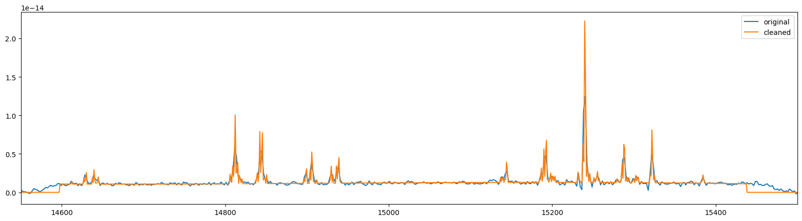
cleaned_spectrum = spectrum.clean(precision=100, threshold=None, cleaned_ils='gaussian', oversampling=2)

pl.figure(figsize=(20,5))
pl.plot(spectrum.axis.data, spectrum.data.real, label='original')
pl.plot(cleaned_spectrum.axis.data, cleaned_spectrum.data.real, label='cleaned')
pl.legend()
pl.xlim(14550, 15500)

master.e47f|INFO| CFHT version
master.e47f|INFO| Cube is level 2.5
master.e47f|INFO| shape: (2048, 2064, 847)
master.e47f|INFO| wavenumber calibration: True
master.e47f|INFO| flux calibration: True
master.e47f|INFO| wcs calibration: True

(14550.0, 15500.0)

Example on a simulated spectrum

This part can be used for testing purpose

import orb.sim

# simulate a spectrum
Interf = orb.sim.Interferogram(500, params='SN3')
Interf.add_line('Halpha', flux=2)
Interf.add_line('Halpha', flux=2, vel=140)
Interf.add_line('[NII]6548', flux=0.5)
Interf.add_line('[NII]6584', flux=0.3)
interf = Interf.get_interferogram()
spectrum = interf.get_spectrum()

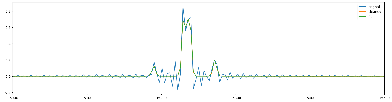
cleaned_spectrum = spectrum.clean(threshold=0.1, oversampling=1)
fit = cleaned_spectrum.fit(['Halpha', 'Halpha', '[NII]6548', '[NII]6584'], fmodel='gaussian', fwhm_def='1', pos_def=['1', '2', '3', '4'], pos_cov=[0,170,0,0])

pl.figure(figsize=(20,5))
spectrum.plot(label='orignal')
cleaned_spectrum.plot(label='cleaned')
fit.get_spectrum().plot(label='fit')
pl.xlim(15000, 15500)
pl.legend()

print(fit)

=== Fit results ===
lines: ['H3', 'H3', '[NII]6548', '[NII]6584'], fmodel: gaussian
iterations: 67, fit time: 4.11e-02 s
number of free parameters: 10, BIC: -3.23296e+03, chi2: 2.54e-04
Velocity (km/s): [-3.176(79) 139.701(95) -3.42(32) -1.37(54)]
Flux: [2.0808(53) 2.0524(55) 0.5260(27) 0.3224(26)]
Broadening (km/s): [nan +- nan nan +- nan nan +- nan nan +- nan]
SNR (km/s): [563.61733295 509.66365136 209.8667744  128.88334292]