Differences between fitting a sincgauss model and two sinc lines

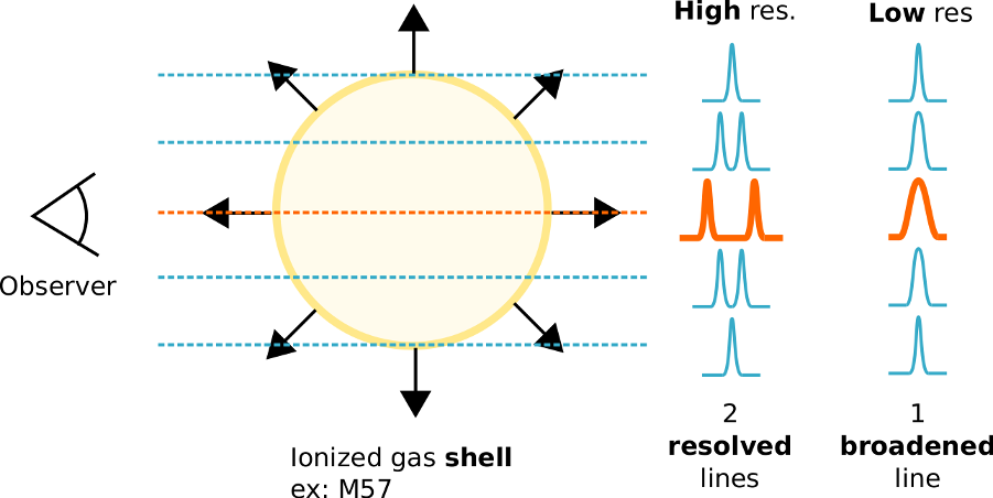
When fitting an unresolved expanding shell both model can be used but we will show that it is generally better to fit the real model : i.e. a model with two sinc lines.

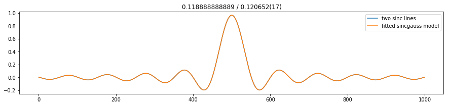
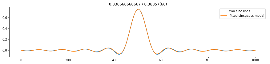
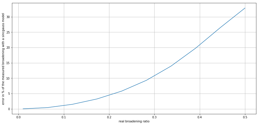
• The broadening measured with a sincgauss line is overestimated by more than 10% when the it is larger than 0.3 times the fwhm (i.e. the resolution)

• The sincgauss model is slow to compute (around 10 times slower than a sinc model, i.e. 5 times slower than a model based on two sinc lines)

%matplotlib inline
import orb.utils.spectrum
import pylab as pl
import orb.fit
import numpy as np

Difference wrt to sigma/fwhm ratio

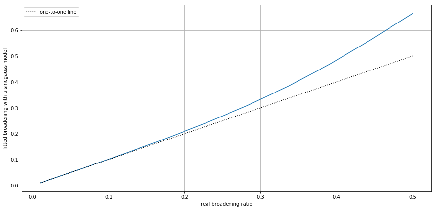
The fwhm is fixed by the resolution. sigma is the expansion velocity. The ratio sigma/fwhm is the ratio of the broadening wrt the resolution. We will show that, at small ratios (sigma < 0.3 * fwhm), it is equal to the broadening of the sincgauss model = the width of the gaussian which is convolved to the sinc. But when the expansion velocity is too high it becomes different.

The following toy model sinc1d_2 is constructed with two sinc lines of equal amplitude.

def sinc1d_2(x, h, a, dx, fwhm, sigma):
    return (orb.utils.spectrum.sinc1d(x, h, a/2., dx + sigma, fwhm)
            + orb.utils.spectrum.sinc1d(x, h, a/2., dx - sigma, fwhm))

# model parameters
x = np.arange(1000)
h = 0
a = 1
dx = np.size(x) / 2
fwhm = 60
sigma = 0.1 * fwhm

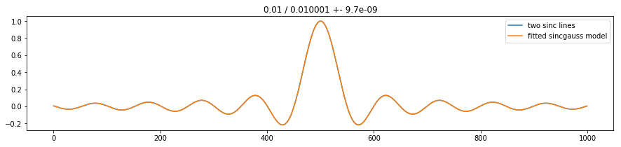
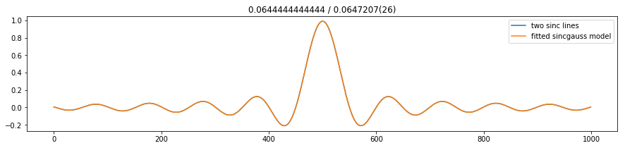
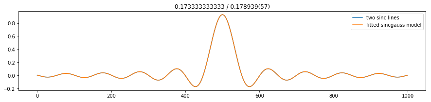
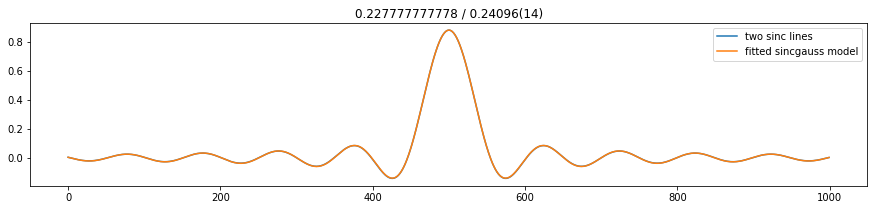
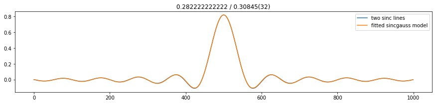
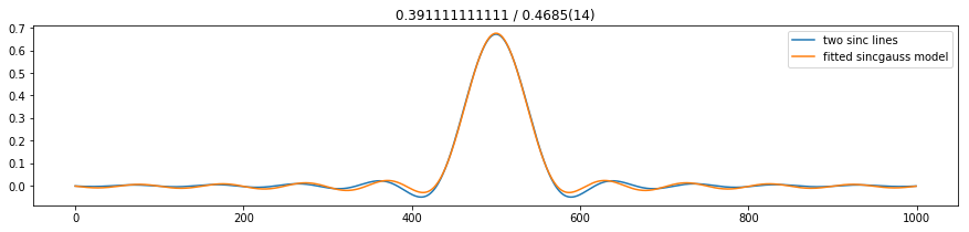
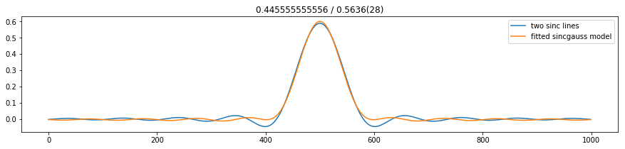
We will now model our unresolved emission lines with the toy model and fit a sincgauss model over it. The title of each graph gives the real sigma/fwhm ratio (in terms of channels size remember that the FWHM is around 1.5 channels with SITELLE).

for isig in np.linspace(0.01, 0.5, 10):
    sd = sinc1d_2(x, h, a, dx, fwhm, isig * fwhm)
    fit = orb.fit.fit_lines_in_vector(sd, [dx], fwhm, fmodel='sincgauss',
                                      sigma_guess=isig*fwhm)
    pl.figure(figsize=(15,3))
    pl.plot(sd, label='two sinc lines')
    pl.plot(fit['fitted_vector'], label='fitted sincgauss model')
    pl.legend()
    pl.title('{} / {}'.format(isig, fit['lines_params_gvar'][0,-1]/ fwhm))

/home/thomas/Astro/Python/ORB/Orb/orb/fit.py:142: UserWarning: No SNR guess given. Fit mode is classic.
  warnings.warn('No SNR guess given. Fit mode is classic.')

real_ratios = list()
fitted_ratios = list()
for isig in np.linspace(0.01, 0.5, 10):
    sd = sinc1d_2(x, h, a, dx, fwhm, isig * fwhm)
    fit = orb.fit.fit_lines_in_vector(sd, [dx], fwhm, fmodel='sincgauss',
                                      sigma_guess=isig*fwhm)
    real_ratios.append(isig)
    fitted_ratios.append(fit['lines_params'][0,-1]/ fwhm)
real_ratios = np.array(real_ratios)
fitted_ratios = np.array(fitted_ratios)

pl.figure(figsize=(15,7))
pl.plot(real_ratios, fitted_ratios)
pl.plot(real_ratios, real_ratios, c='0.', ls=':', label='one-to-one line')
pl.xlabel('real broadening ratio')
pl.ylabel('fitted broadening with a sincgauss model')
pl.legend()
pl.grid()

pl.figure(figsize=(15,7))
pl.plot(real_ratios, (fitted_ratios-real_ratios)/real_ratios * 100)
pl.xlabel('real broadening ratio')
pl.ylabel('error in % of the measured broadening with a sincgauss model')
pl.grid()